What is it all about?
We’re using a bunch of VMs to do numerical dosimetry and are very satisfied with the service and performance we get. Here I try to give some background on our work.
Assume yourself sitting in the dentists chair for an x-ray image of your teeth. How much radiation will miss the x-ray film in your mouth and instead wander through your body? That’s one type of question we try to answer with computer models. Or numeric dosimetry, as we call it.
The interactions between ionizing radiation – e.g. x-rays – and atoms are well known. However, there is a big deal of randomness, so called stochastic behavior. Let’s go back to the dentists chair and follow one single photon (that’s the particle x-rays are composed of). This sounds a bit like ray tracing, but is way more noisy as you’ll see.
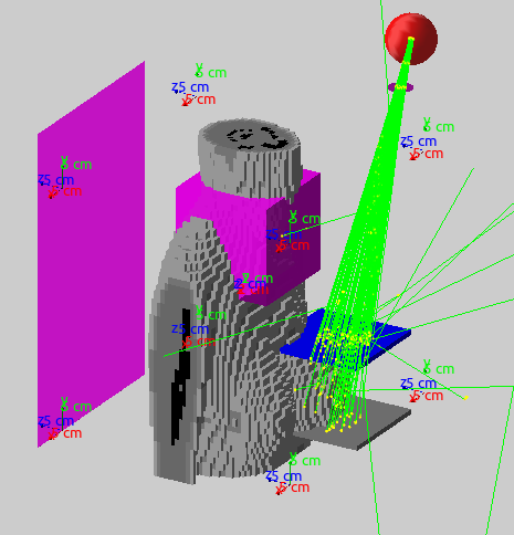
The image below shows a voxel phantom (built of Lego bricks made of bone, fat, muscle etc.) during a radiography of the left breast.
Tracing a photon
The photon is just about to leave the x-ray tube. We take a known distribution of photon energies, throw dices and pick one energy at random. Then we decide – again by throwing dices – how long the photon will fly until it comes close to an atom. How exactly will it hit the atom? Which of the many processes (e.g. Compton scattering) will take place? How much energy will be lost and in what direction will it leave the atom? The answer – you may have already guessed that – is rolling in the dice. We repeat the process until the photon has lost all it’s energy or leaves our model world.
During its journey the photon has created many secondary particles (e.g. electrons kicked out of an atomic orbit). We follow each of them and their children again. Finally, all particles have come to rest and we know in detail what happened to that single photon and to the matter it crossed. This process takes some 100 micro seconds on an average cloud CPU.
Monte Carlo (MC)
This method of problem solving is called Monte Carlo after the roulette tables. You always apply MC if there are too many parameters to solve a problem in a deterministic way. One well know application is the so called rain drop Pi. By counting the fraction of random points that are within a circle you can approach the number Pi (3.141).
Back to the dentist: Unfortunately, with our single photon we do not see any energy deposit in your thyroid gland (located at the front of your neck) yet. This first photon passed by pure chance without any interaction. So we just start another one, 5’000 a second, 18 Millions per hour etc. until we have enough dose collected in your neck. Only a tiny fraction q of the N initial photons ends up in our target volume and the energy deposit shows fluctuations that typically decrease proportional to 1/sqrt(qN). So we need some 1E9 initial photons to have 1E5 in the target volume and have a relative error smaller than 1 %. This would take 2 CPU days.
MC and the cloud
This type of MC problems is CPU bound and trivial to parallelize, since the photons are independent from each other (remember that in a drop of water there are 1E23 molecules, our 1E9 photons will not disturb that). So with M CPUs my waiting time is just reduced by a factor M. In the above example and with 50 CPUs I have a result after 1 hour instead of 2 days.
This is a quantitative progress on the one hand. But on the other hand and more important for my work is the progress in quality: During one day, I can play with 10 different scenarios, I can concentrate on problem solving and do not waste time unwinding the stack in my head after a week. The cloud helps to improve the quality of our work.
Practical considerations
The code we use is Geant4 (geant4.cern.ch), a free C++ library to propagate particles through matter. Code development is done locally (e.g. Ubuntu in a virtual box) and then uploaded with rsync to the master node.
Our CPUs are distributed over several virtual machines deployed in ICCLab’s OpenStack cloud. From the master we distribute code and collect results via rsync, job deployment and status is done through small bash scripts. The final analysis is then done locally with Matlab.
Code deployment and result collection is done within 30 seconds, which is negligible compared to run times of hours. So even on the job scale our speedup is M.