How reliable are your OpenStack VMs? How many outages do you expect to occur during 8 months of operation? Do your VMs crash regularily, randomly or do VM outages increase over time? These questions can only be answered if we perform a reliability analysis of the virtual machines that we manage. In this small guide we show you how to check reliability of VMs in your OpenStack environment. In part 1 of this 4 part series we explain the basic concepts of reliability engineering.

The vast field of reliability engineering has been used widely in various engineering disciplines like aircraft design, civil engineering, electricity management or product management. Though reliability engineering has proven to help in successfully building high quality engineering products, it has almost never been used in cloud computing so far. There might be some distrust among programmers in these scientifically proven reliability analysis methods, since they involve math and statistical exploration. But with a little introduction this is not a severe problem that we should worry about.

Reliability engineering simply deals with analyzing and measuring the outage behavior of engineered systems, trying out and testing system improvements that make the system more reliable, implementing system improvements and validating if the system improvements have reduced the occurence of outages or not. The first step is the analysis of outage behavior. How can outages be analyzed?

Why do virtual machines fail?

Let us start with a small thought about outages: why can your virtual machine just crash without any warning sign? At least it is just a software that emulates a physical computer – it is just an algorithm! How can a piece of logic just fail?

The answer is that even virtualization software is more than just a piece of logic code. First it runs on a computer which is a physical artefact and therefore subject to various physical forces (electricity, heat) that could possibly damage it. Second it is programmed by humans who are notoriously making mistakes all the time. And third: even if we assume that the virtual machine is programmed correctly and it runs on an extremely reliable server – how can we make sure that the user of the VM is operating it correctly?

Outages occur randomly

As we might see: outages just occur randomly. Even virtual appliances like OpenStack VMs fail randomly and even more often than physical machines. In reliability engineering we assume that outages occur at random and that we have to measure these randomness to gain insight in the behavior of these outages.

It is rather paradox to measure something that occurs at random and at the same time expecting that measuring it would make any sense. How can we say now that it makes sense to measure outages if they appear so randomly? The reason for that is simple: “randomness” follows rules. And these rules help us to understand the outage behavior of virtual machines.

Hazard rate and hazard function

If you throw a coin it will either flip on heads or tails side. The probability for either side is 0.5 or 50%. For each throw this probability stays uniform. The probability of throwing heads in the next throw is independent of the result of previous throws. It follows the simple rule that the probability for either side is always 0.5.

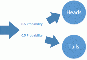
Throwing a coin multiple times is a series of discrete events. This the system we observe has always a clearly defined state. Now think of a server running in a data center: this system does not have discrete states, it is operating continously.

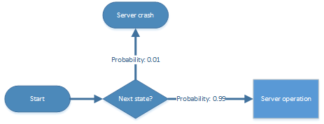
The only “discrete event” that could occur would be a server crash or another event leading to an outage. How should the probability of such an event be described? Here we introduce the term of the “hazard rate”. The hazard rate is the probability that the observed system will fail in the next time unit.The probability that the system will survive the next moment is called the survival rate. At any moment in time the server is facing a similar coin flipping game: either the server survives the next time step or it does not. The probability of the later is the hazard rate. The probability of the other outcome is called the “survival rate”.

The survival rate is simply the “complementary” probability of the hazard rate. Its value is 1 minus the value of the hazard rate. If you add both rates to each other the result is always 1. If the hazard rate is e. g. 0.01 or 1%, the survival rate must be 0.99 or 99%.

The operation of the server could be seen as a series of infinitely many time steps or discrete events. Every operation step of the server is like throwing a coin: the hazard rate is the probability that the server will fail in the next instant and the survival rate is the probability that the server continues its operation. The server operation is an infinite series of such coin tosses that decide wether the server will continue its operation or not.

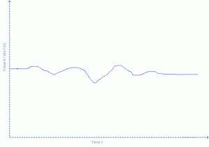
When we model the operation of a computer as a series of infinitely many discrete events that occur in time, we could draw a function of hazard rate values versus the time when the given hazard rate value is valid. This function of time dependent hazard rates is continuous and because it is a function that shows how the hazard rates are distributed over time interval it is called a “hazard function”. Random events like outages follow a hazard function h(t) which tells you how likely it is that the outage might occur in the next instant of time.

Failure rate

The hazard rate is an “instantaneous” probability: it is valid only for an infinitely small point in time. In practice we are not able to measure it, because measuring takes time and we can measure only outages that occur in a given time interval. Therefore we introduce the term “failure rate”. The failure rate f(t) is the probability that an item will fail during the next time interval t. It is measured in failures per time unit (e. g. failures per hour).

Consider a number of virtual machines in OpenStack. We observe our cloud environment  for 5’000 hours (about 7 months) and check if our VMs are still alive every hour. at the beginning there are 100 VMs up and running. After 5’000 hours we see that one VM has crashed, 99 VMs are still alive. The failure rate for t=5’000 is then 1/100 failures per hour.

Failure probability

The failure rate is useful information, but it is quite a bad predictor, because it increases only after the VM has crashed. We might be more interested in the probability that a VM crash occurs within a given time frame. Therefore we introduce the failure probability F(t) which is the probability that a system fails during a given time frame.

In the former example we checked the VMs every hour. Now we take only two measurements: one at the beginning, where all 100 VMs are up and running and one at t=5’000 hours, where the first VM has crashed. We conclude that for the time frame of 5’000 hours there is a 1% probability of failure, since 1% of the VMs have crashed. F(t) is 0.01 or 1%.

Now consider that we wait 5’000 hours more. After 10’000 hours there are only 95 VMs still alive. If we would measure the failure rate every hour we would see that the failure rate f(t) has increased during this 5’000 hours to 4/100 failures per hour. The failure probability for 10’000 hours has also increased, but it is now 0.05 or 5%.

The failure probability F(T) is simply the integral of failure rates f(t) during the interval of time t from 0 to T.

Reliability

As system administrators we might have gathered now the evidence that after the first VM has crashed, there is a 1/100 probability that a VM might crash in the next hour. This is useful information but if we want to plan maintenance actions we might also be interested in how long does it take until we have to start with maintenance operations. We want to know the probability of a VM to survive a given time frame t. The propability R(t) of an item to survive until time t is called “reliability”.

Consider again that we have 100 OpenStack VMs running for 10’000 hours. After 10’000 hours 95 VMs are still up and running. The reliability for t=10’000 is then 0.95, because 95 % of the VMs survived for 10’000 hours.

Reliability R(t) is simply the complementary probability of the failure probability F(t).

Connection between hazard rate, failure rate and reliability

How can we exploit the given measurements to calculate the hazard rate? The hazard rate is instantaneously formed during a given time interval. We define the hazard rate h(t) as the ratio between failure rate f(t) and reliability R(t).

Since reliability R(t) is the complementary probability to the failure probability F(t) and F(t) is the integral of f(t), the hazard rate h(t) can be computed as soon as either R(t), F(t) or f(t) is known.

Probability density function of failure rates

If we draw the values of f(t) in a diagram showing the failure rate in dependency to the time, we get the “probability density function”, a function that explains how the failure rates are distributed over a time interval. Outages are random events that follow the distribution expressed in the probability density function. Typical distributions of outage probabilities are the exponential distribution and the Weibull distribution.

Exponential distribution

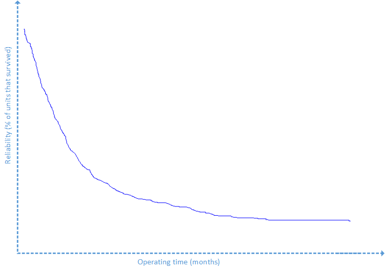
The exponential distribution is shaped by the parameter λ. λ is the expectation value as well as the standard deviation of the exponential distribution. The following equations are characteristic to the exponential distribution:

An important characteristic of the exponential distribution is that the hazard rate is constant. The following equation proves that.

Having a constant hazard rate means that the exponential distribution has “no memory”: if the system has not failed after 10’000 hours of operation the probability of failure in the next instant of time is equal to the same probability after 20’000 hours of operation.

Since software is not a physical artefact and therefore not subject to physical deterioration its failure rates should (theoretically) be exponentially distributed.

Weibull distribution

The assumption of constant hazard rates may be an oversimplification. Computer users may know it from their own experience: new software is extremely buggy in the first version and slowly becomes more and more stable when it is patched as it gains maturity from version to version.

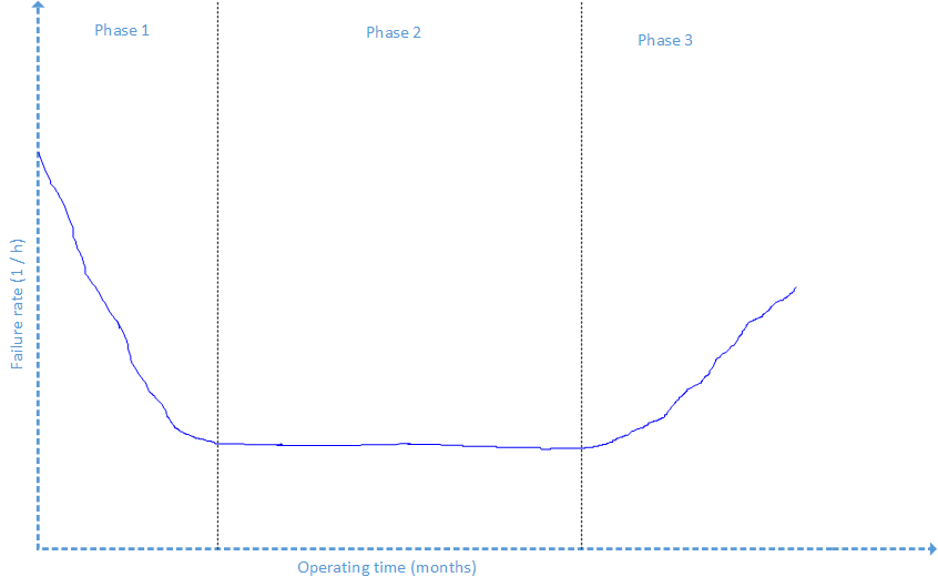
The hazard rates of software are normally not constant. They follow rather a “bathtub” shaped curve. Usually new software which is shipped contains lots of bugs and crashes extremely often. It becomes more and more stable when it is patched later on and the hazard rate begins to drop. The hazard rate drops from patch to patch until it reaches its bottom. In that phase hazard rates may be low and nearly constant. After being on the market for 3-4 years the software faces more errors. Security leaks are detected, patches are uploaded, but changes of the software become difficult. The hazard rate climbs up again until the software support is discontinued because there is something newer on the market.

The bathtub curve has three phases: a phase with declining hazard rates, a phase with constant hazard rates and a phase with increasing hazard rates. A failure rate function which models the bathtub curve is called the “Weibull” distribution.

The Weibull distribution knows two parameters:

• The scale parameter α
• The shape parameter β

The characteristic equations of the Weibull distribution are:

Next post: find out how to apply this to OpenStack VMs

In the introduction to this article we mentioned that we want to get to know more about the reliability engineering. The first step consists in analyzing realibility parameters: we have to find out the distributions of f(t), F(t), R(t) and h(t).

In the next blog post of this series we will explain how to do this for a bunch of OpenStack VMs by using Python, fabric and R.