By Oliver Dürr (ZHAW)
Reposted from http://oduerr.github.io/blog/2016/04/06/Deep-Learning_for_lazybones
In this blog I explore the possibility to use a trained CNN on one image dataset (ILSVRC) as feature extractor for another image dataset (CIFAR-10). The code using TensorFlow can be found at github.
Background
Image classification has made astonishing progress in the last 3 years. While 2012 a computer could hardly distinguish a cat from a dog, things have dramatically changed after [Alex Krizhevsky et al., 2012] won the Imagenet classification competition using a deep learning method called convolutional neural network (CNN).
They achieved a top-5 error rate of 17% compared to 26% of the second best approach. While back in 2012 one had to be a hard core C++ programmer to build and train these models, recently several new deep learning frameworks have emerged: e.g. Theano, Lasagne, Torch. They make it possible to use deep learning if you know just some python. In November 2015 Google released their own framework called TensorFlow with much ado. Recently, a network termed inception-v3 trained on the ILSVRC-2012 dataset has been made publicly available for TensorFlow [Szegedy et al, 2015]. This network achieves an astonishing top-5 error rate of 3.6%. Given the fact that humans achieve approximately 5% (partly due to the 120 different breeds of dogs in the data set) this is very amazing.
Doing image classification on your own data
What to do if you want to apply this network on your own image classification task? You have the following options:
- If you have enough labeled data (the ILSVRC-2012 competition has 1000 classes and 1 million training examples), you could take the architecture of the network and train it from scratch. This would take 2 weeks on (very) decent hardware.
- If you have less data, you could fine-tune the network on your classes. This is called transfer learning and described e.g. in the TensorFlow tutorial. But this approach still needs quite some time and you have to train a deep neural network.
- If you have just some data and not much time to spend for training a CNN, could you just use the CNN to create features as input for a ‘classical’ machine learning approach, e.g. a support vector machine (SVM)?
In this post we want to elaborate on method 3 using python and TensorFlow. The code (less than 50 lines) can be found on github. Of course this is not a new idea, a similar approach has been described in [Jeff Donahue et al., 2013].
The test data:
How well does this easy choice work? To test this approach, we use the CIFAR-10 dataset, which can be obtained from here. Note that the model has been trained on ILSVRC-2012 images, which is a different dataset than CIFAR-10. Here are some examples of the data-set with the following 10 classes: airplane, automobile, bird, cat, deer, dog, frog, horse, ship, and truck displayed as rows:
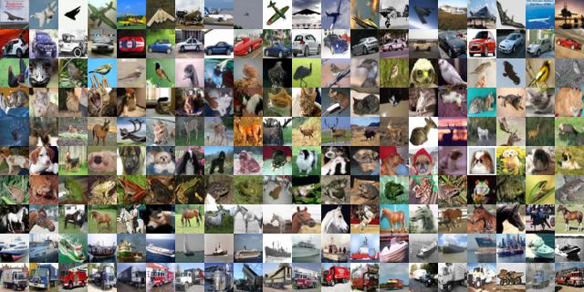
Note that the ‘inception v3’ can deal with images of size 299×299, without the need of downscaling them. So using the tiny 32×32 images from CIFAR-10 is quite an overkill.
Extracting the features using the CNN network
Which layer to use? The network to has been trained for the 1000 classes of the ILSVRC-2012 dataset but instead of taking the last layer – the prediction layer – we use the penultimate layer: the so-called 'pool_3:0’ layer with 2048 features. This layer can be regarded as a representation layer, which represents images as 2048 dimensional feature vectors.
Technically: all we have to do is to pass the images into the trained graph. We use the routines maybe_download_and_extract() to possibly download the trained network and create_graph() to create an instance of the trained model. These methods are provided in the file 'classify_image.py', which we just copied from the TensorFlow repository. A subtlety, which took me some time to understand, is that if you have images as a numpy arrays with dimension say (32,32,3) and not a jpeg-string you have to feed it into a confusingly termed node 'DecodeJpeg:0'. I found this solutions in a stack overflow answer. A side note: If you have image encoded in a jpg format you could use the 'DecodeJpeg/contents:0’ layer, as described in the Googles tutorial. What is very convenient in any case, is that you do not need to bother about scaling and normalisation, this all happens in the TensorFlow graph. Here are the important commands to extract the features:
from classify_image import *

...

FLAGS.model_dir = 'model/'

maybe_download_and_extract()

create_graph()

with tf.Session() as sess:

representation_tensor = sess.graph.get_tensor_by_name('pool_3:0')

...

for i in range(len(y)):

...

[reps, preds] = sess.run([representation_tensor, softmax_tensor], {'DecodeJpeg:0': imgs[i]}) #imgs (10000,32,32,3)

...
The full code is available in the python script cifar-10_experiment.py. To run the code check out the repository, download the python version of the CIFAR images extract them and place them into a directory. Change the path in cifar-10_experiment.py line 13 to that directory. Run the script in checkout repository (directory tensorflow/inception_cifar10).
(venv)dueo@deepfish:~/dl_tutorial/tensorflow/inception_cifar10 python cifar-10_experiment.py
This script will download the TensorFlow model and does the feature extraction for the CIFAR images. This script needs about 0.03 seconds per image on a Titan X GPU, and on my 13’’ Late-2013 MacBook Pro it takes approximately 0.5 seconds on the CPU. I guess the code could be further enhanced using batches instead of feeding in one image after another, but I want to keep it simple.
Doing the classification
That’s pretty straight forward, see the Analyse_CIFAR-10_Classification.ipynb. After loading the features, we train a SVM on batch 1 of the training data set (note that we don’t even use the whole training set and don’t use the batches 2 to 5). Then we do a prediction on the 10000 images on the test-set with:
svc = svm.SVC(kernel=’linear’, C=0.1).fit(rep_train,y_train)

res = svc.predict(rep_test)

np.sum(res == y_test)/10000.0 #0.8741
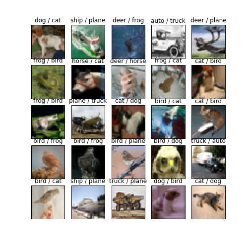
If we compare this with the state-of-the-art results, the 87% we achieve are not bad at all, considering the fact that we did not need to train the network but just a SVM. If you used, for example HOG-features, you would get about 59%. In my opinion this shows that using hand-crafted features like HOG does not make much sense anymore, we reduced the error from 41% down to 23% by simply using a trained network for feature generation. For illustration, here are some examples for which we have been wrong, some of these mistakes are quite obvious:
Bonus: t-SNE visualization
For visualization purpose, one could also use the extracted features for the 10’000 images of the test set (we could have also used the training set of course). On this 10000×2048 matrix, we do a t-SNE dimension reduction to 10000×2 and visualize it in a scatter plot. Note that t-SNE is a purely unsupervised method and that we do not use the labels besides for coloring after the analysis. See Analyse_CIFAR-10_TSNE.ipynb for the code and here for the full sized image of the result. See also t-SNE visualization of CNN codes for similar visualisations of the ILSVRC-2012 dataset, from where I got the visualisation idea.

tl;dr
We use the trained (on ILSVRC-2012) inception v3 network available in TensorFlow to extract features from CIFAR-10 images. Using a simple SVM, we get very acceptable classification results. We further show how these features could be used for unsupervised learning. Code is available on github.